From Bayesian inference to modern machine learning

< Previous post

Epistemic status: I’m not an expert on many of the machine learning methods mentioned, and the discussion is primarily conceptual. Expect some abuse of notation. I will use the word ‘true’ a lot, which here means something along the lines of ‘corresponding to actual states of the universe’.

In the previous post we discussed how objective Bayesian inference prescribes using Bayes' theorem to learn about the world: $p(\mathcal{H}|\mathcal{D},\mathcal{I})=\frac{p(\mathcal{H}|\mathcal{I})p(\mathcal{D}|\mathcal{H},\mathcal{I})}{p(\mathcal{D}|\mathcal{I})}$.

This first requires specifying a specific prior distribution $p(\mathcal{H}|\mathcal{I})$ over all (possible) hypotheses $\mathcal{H}$ given your prior information $\mathcal{I}$. This prior defines an inductive bias on the inference problem, and all that remains is to observe data $\mathcal{D}$, compute the likelihood $p(\mathcal{D}|\mathcal{H},\mathcal{I})$ for all hypotheses $\mathcal{H}$ (typically specified by $\mathcal{H}$ itself), and finally use Bayes' theorem to obtain the posterior distribution $p(\mathcal{H}|\mathcal{D},\mathcal{I})$, which represents the unique correct description of your current state of information about the world.

We already noted how staggeringly impossible this is to do exactly, and thus any kind of Bayesian inference done in practice involves approximations. The common modern machine learning recipe - of specifying a parameterised model class, some prior (or no prior!) over these parameters, and using data and some learning rule to update these parameters so that they minimise some risk function - is precisely such an approximation. Here we will see how.

Let’s start slowly: we’ll adhere to the general Bayesian idea that we need some kind of posterior distribution to describe our state of knowledge of some process, but we make some approximations in how we compute this.

Exact inference

The simplest case is the ‘exact inference’ setting, where we can actually compute the evidence term $p(\mathcal{D}|\mathcal{I})=\int p(\mathcal{H}|\mathcal{I})p(\mathcal{D}|\mathcal{H},\mathcal{I})d\mathcal{H}$ exactly. This might for instance be the case when we’re talking about computing a posterior $p(\mu |\mathcal{D},\mathcal{I})$ for the mean $\mu$ of a Normal distribution given some data and a known standard deviation. If we use a conjugate prior for $\mu$, then the posterior can be exactly computed, so we’ve done exact inference! Right?

The model choice

Well, note that we just introduced the Normal distribution out of the blue. If we were proper Bayesians, we would instead have started by considering a distribution over possible hypotheses $\mathcal{H}$ consistent with our initial information $\mathcal{I}$. These hypotheses then immediately define their corresponding likelihood $p(\mathcal{D}|\mathcal{H},\mathcal{I})$. Indeed, that’s what an hypothesis is: it tells us precisely what kind of data we expect to see. In the above example, we’ve decided to only care about hypotheses that expect our observations to be Normally distributed with a fixed standard deviation around some particular $\mu$, and the value of this $\mu$ is the only thing that distinguishes one hypothesis from another. What if reality is more complicated? Well, then we will not discover this, because we haven’t included those options in our hypothesis class.¹ This is a very strong approximation.

In the language of inductive biases, we’ve biased our inference to only caring about explanations that are described by a Normal posterior. We will find the best explanation of our observations within this class, but we will not find the true explanation if our hypothesis class does not contain it. Of course, if our current information $\mathcal{I}$ says that - out of all potential hypotheses - only Normal hypotheses with this particular standard deviation are are possible, then we’re following the Bayesian prescription; we are then, in fact, considering all hypotheses consistent with our information. We might ask ourselves, however, whether we are ever in possession of such an $\mathcal{I}$.

The prior

Now let’s have a look at the chosen prior $p(\mu |\mathcal{I})$ as well. We used conjugate priors so that we were able to evaluate the evidence, but this was motivated only as a convenient mathematical trick: to what degree does such a prior actually describe what our current information $\mathcal{I}$ tells us about $\mu$? The conjugate prior for a Normal distribution with fixed standard deviation is another Normal: when is this a good prior?

A full answer would take us on a trip down the rabbit hole of constructing objective prior distributions, which is one of the hard problems mentioned in the previous post. One interesting result, though, is that the Normal prior can be motivated through the principle of maximum entropy as the prior that uniquely encodes knowledge of the first and second moment of a parameter, and no other information. So, if we already have some vague idea of the magnitude of $\mu$ and of how far we might be off, then the Normal prior is a pretty good choice: not ideal, but a fairly good description of $\mathcal{I}$.

The ‘exact’ inference setting we looked at here is an insightful one to consider first, since its approximations - using a constrained hypothesis class and choosing a prior that might not fully reflect all known information - come up in (as far as I know) all practical inference methods. Going beyond the exact inference setting - towards settings where we cannot evaluate the evidence term - necessitates additional approximations. Let’s look at some of these non-exact methods now.

Non-exact inference

Two widely used inference methods in modern day Bayesian deep learning are Markov Chain Monte Carlo (MCMC) and Variational Inference (VI). They typically involve more complex hypotheses than those used in exact inference, which means the evidence term cannot be exactly evaluated. Both of these methods try to solve the intractability of the evidence term by introducing an approximation. The below is a brief discussion on the types of approximations these methods make to the prescription of Bayesian inference: see the above links for a starting point on a more thorough explanation of the methods.

Markov Chain Monte Carlo

MCMC tries to generate samples from the posterior by setting up a Markov Chain whose stationary distribution is the posterior. The set-up avoids having to evaluate the evidence, since the chain can be constructed using the ratio of the posterior at any two points, and the evidence term cancels out in this ratio.

So what are the approximations? First of all, there are the same hypothesis space and prior approximations we saw in the exact inference case: we typically consider a restricted set of hypotheses, and our choice of prior might not reflect our information exactly. Secondly, the chain generates samples of the posterior. Even if the sampling is from the exact posterior specified, any finite number of samples is not going to be an exact match for that posterior. Thirdly, samples might not be exactly from the posterior specified due to convergence issues with the chain. Most improvements to vanilla MCMC methods focus on tackling this last problem, as well as on speeding up inference, which can be quite computationally intensive.

Variational Inference

VI essentially turns the original inference problem into an optimisation problem. It tries to approximate the posterior by varying the parameters of another proposed distribution until it fits the posterior adequately. The approximating distribution is chosen from a relatively tractable family of distributions, to simplify the procedure. The actual optimisation is typically performed on a lower bound of the evidence term, which has the intended effect of squeezing the approximate distribution closer to the specified posterior.

Beyond the two standard approximations of practical Bayesian inference, VI introduces an approximation on the specified posterior, which is then fitted by optimising an approximate objective: two more approximations!

It’s quite difficult to characterise the effect of the MCMC and VI approximations on the inductive bias of the inference process.² Their hypotheses classes are typically less restrictive than those used in exact inference, but their convergence dynamics may play a large role in the kind of inferences that pop out.³

Although MCMC and VI introduce quite some approximations, they are two of a relatively rare class of methods that attempt to obtain something that looks like a Bayesian posterior.⁴ Most modern machine learning methods don’t do this, so let’s see how we can obtain them from the Bayesian prescription.

Through decision theory to maximum likelihood

In the previous post, we saw that by Cox’s theorem our state of knowledge of the world can be described by a probability distribution over all possible hypotheses consistent with our available information. We can then learn from observations through Bayes' theorem, and fundamentally that’s all there is to inference: as we said, all the rest is commentary.

So how do we get the most common modern day machine learning practice - training some model to maximise its likelihood - from this prescription? The answer lies in decision theory.

Decision theory

Maximising a likelihood function just returns a single parameter value: the parameter setting that best explains the observed data according to that likelihood function. This is a far cry from the full posterior distribution that we need to describe all our information: we’ve thrown away information to make our lives easier.

By describing our state of knowledge now with a single parameter value plus some pre-specified model, we have chosen a particular summary of our full state of information. Which summary we choose is a decision we make - they all throw away some information, but different summaries throw away different information - and we will see that the maximum likelihood solution corresponds to one such summary. Whether this choice is a good one really depends on what we want to achieve. Bayesian inference tells us what we know, it doesn’t tell us what we care about: it’s the role of decision theory to formalise the kind of trade-offs we’re willing to make.

Deriving MLE from Bayes

So, how do we describe this formally? We are trying to summarise our posterior distribution $p(\mathcal{H}|\mathcal{D},\mathcal{I})$ using some single statistic $S$. Any summary will discard some information, and we can define a decision loss function $L(\mathcal{H},S)$ that tells us how much we care about certain information versus other information contained in the full posterior. In other words, this loss function tells us how bad it is to use a particular statistic $S$ in the case that $\mathcal{H}$ is the true hypothesis, and it does this for all hypotheses we’re considering. There is some abuse of notation here, so let’s say this another way: given some summary statistic $S$, we check for each possible hypothesis $\mathcal{H}$ how bad it would be if we made a decision based on $S$ if $\mathcal{H}$ were true (here - for simplicity - each $S$ directly corresponds to a decision).

As an example, let’s say we’re considering hypotheses on the probability of earthquakes within the next ten years. Instead of using our full posterior to describe this, we choose to use the most likely hypothesis - according to our posterior - as our summary statistic $S$.⁵ If this is also the true hypothesis then we’ve presumably made a good choice, since we’ll be making decisions based on something true. If not, then we’re making decisions based on something false, and in particular we’re throwing away almost all information contained in the posterior distribution that might tell us how wrong we are. In the context of earthquakes, we’d be basing our decisions purely on the (potential) summary ‘the most likely earthquake in the next ten years will happen in Japan’. This discards very little information if our actual posterior says there is very low probability on hypotheses that there will be earthquakes somewhere else in the next ten years; otherwise, we’ve thrown away a lot.

So how bad do we expect such a decision to be? Well, our posterior exactly represents our belief over these various earthquake possibilities, so the expected badness can be computed as the expectation of the loss under our posterior distribution. We write ${\mathbb{E}}_{p(\mathcal{H}|\mathcal{D},\mathcal{I})}L(\mathcal{H},S)$ for this expectation, and we want to minimise this expected loss over decisions, which here directly correspond to choices of statistics $S$.

Following the example above, let’s see what happens if we decide use a loss function that assigns loss 0 if $S=\mathcal{H}$ and 1 otherwise, writing this as $1-\delta (\mathcal{H},S)$, where $\delta (.)$ is the delta function.⁶ This loss function cares about exactly choosing the correct hypothesis; and if we’re wrong, then we don’t care how wrong we are. Intuitively, this choice will make us pick the most likely hypothesis as our summary, since it has the highest probability of being correct given our current information.

Minimising this expected loss over choices of $S$ is all we need to obtain the maximum likelihood formalism:

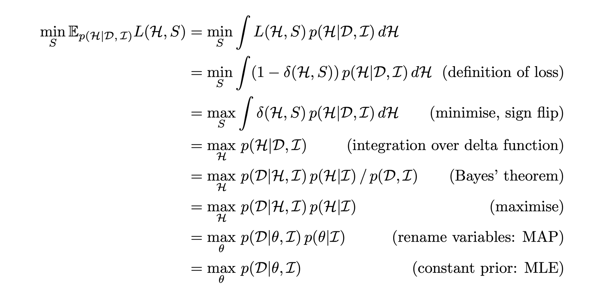
Here we have renamed $\mathcal{H}$ to $\theta$ to make the correspondence with typical Maximum A Posteriori estimation (MAP) and Maximium Likelihood Estimation (MLE) clearer. Typically when we write $\theta$ we are referring to the parameters of some model, and in principle $\mathcal{H}$ is more general than this, but in the case that we are working within some predefined model class - a linear model, a neural network - the correspondence is exact.

The upshot: the common MLE recipe of machine learning is exactly Bayesian inference with a restricted hypothesis class, a (constant) uniform parameter prior, and a choice to only care about the most likely hypothesis / parameter value, with no extra care as to how wrong we might be. The advantage: it’s a lot easier than full Bayesian inference.

What to do with MLE

So where does this leave us? The ubiquity of Maximum Likelihood Estimation in modern machine learning practice might seem worrying in light of this derivation: how can we expect to make useful decisions based on our models, if they throw away so much information, and take a such a risky approach to decision theory?

Part of the answer is that we can’t and we shouldn’t: for many applications uncertainty estimates are very important, and these are simply not provided by MLE methods. To mitigate this, we can do robustness and calibration analyses that give us some idea of how important the discarded information is for the predictions we intend to use our models for. In the end, the applicability of and MLE model is determined by what our posterior looks like: if it’s very peaked around the MLE hypothesis, then we might be fine, but this is of course hard to tell without access to the full posterior.

Additionally, we haven’t discussed some important complexities surrounding prior information. The MLE formulation doesn’t talk about priors explicitly, but the above shows that it implicitly uses a uniform prior over the parameters. This is far from the full story however, as in practice a lot of our prior information enters as modelling choices, which induce their own kind of inductive bias: more on this in the next post.

Next post >