Priors and generalisation
Implicit priors in deep learning methods
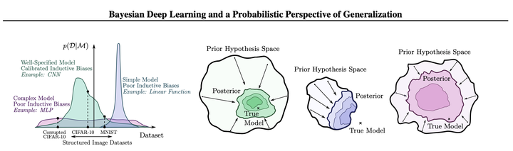 Image by Andrew Wilson and Pavel Izmailov
Epistemic status: lots of handwaveyness connecting our prior knowledge to our ML design choices.
I really like the above figure, taken from Andrew Wilson’s and Pavel Izmailov’s insightful paper Bayesian Deep Learning and a Probabilistic Perspective of Generalization (2020). It conceptually shows the importance of choosing a model’s inductive biases for doing inference in modern imaging tasks: choose the range of observations your model can explain too narrowly and you might miss the ‘true’ model, choose it too widely and your network needs too much data to learn (in the best case). Let’s look at this inductive bias more closely.
(The paper itself primarily discusses the advantages of Bayesian marginalisation in modern neural networks – which is not our current topic – and well worth a read for all who have an interest in Bayesian deep learning.)
Inductive biases
In previous posts we discussed the Bayesian prescription for inference. In this prescription, the prior $p(\mathcal{H}|\mathcal{I})$ over the hypothesis space $\mathcal{H}$ of all hypotheses consistent with your available information $\mathcal{I}$ is the only place inductive biases enter. These hypotheses each directly define a likelihood function $p(\mathcal{D}|\mathcal{H}, \mathcal{I})$ over observations $\mathcal{D}$, and Bayes' theorem tells us how to then compute the posterior $p(\mathcal{H}|\mathcal{D}, \mathcal{I})$ that uniquely describes our state of information about the universe.
Constrast this to modern machine learning practice, where we often don’t talk about priors at all. And yet, we speak of our models as still containing various inductive biases. We say a standard Convolutional Neural Network (CNN) has better inductive biases for image data than a Fully-connected Neural Network (FNN), even when we’re training these models through Maximum Likelihood Estimation (MLE), with no explicit sign of Bayes or priors anywhere.
What’s happening here, is that we are in fact using prior information - in the Bayesian sense - when training these models. It’s just that we’re now so far from the Bayesian prescription that it has become hard to notice. Let’s explore this.
Model architecture as a prior
What is actually happening when we design a deep learning model to solve a particular task? What is our decision process? When working with image data, for a long time the standard choice was to use a CNN (these days you might use a Vision Transformer instead). The reason for this, is that a CNN has a strong inductive bias built in, namely that of translation equivariance. Translation equivariance is the property that translating an input image leads to a similarly translated output: i.e., if an input image has a dog in the top-left, and I shift the image such that the dog is now in the top-right, then the representation of this image in the CNN should also shift such that the CNN activations are the same (just shifted, although not necessarily in the same way as the input image was shifted). What this means, is that our CNN does not have to learn that an image with a dog in the top-left is similar to one with a dog in the top-right; this is built-in to the architecture.
So why would we choose this architecture? We choose this architecture because we know such an inductive bias would help with learning about images. This is because we know that images with top-left dogs are similar to those with top-right dogs, at least for most tasks we’re interested in. We choose this architecture based on our prior knowledge of the problem at hand. A CNN is a prior on the hypothesis space $\mathcal{H}$. In fact, it is such a strong prior that it puts $0$ probability mass on any hypothesis that is not translationally equivariant (up to some details to do with image boundaries). This is actually a too strong prior for most image-related tasks, but it works much better than using fully-connected networks, unless we have access to huge datasets and some more recent tricks.1
We make many more architectural choices when modelling a problem: model depth, data normalisation, optimiser choice, initialisation, etc. These choices are typically based on previous literature, or a practitioner’s intuition: all forms of prior information. And note, even the process of experimenting, evaluating on a validation dataset, and updating the model architecture and optimisation procedure, follows the spirit of Bayes' theorem: updating on evidence to obtain the posterior $p(\mathcal{H}|\mathcal{D}, \mathcal{I})$ and using that as the new prior $p(\mathcal{H}|\mathcal{I})$ for the next round of experimentation.
MLE = MAP
All this means that, in some sense, Maximum Likelihood Estimation is more like Maximum A Posteriori (MAP) estimation in practice. It just doesn’t really happen that we are modelling on the basis of a truly uniform prior over some hypothesis space: every choice we make leaks prior information into the training of our model. And this is good! We’ve previously discussed how the No Free Lunch theorem implies that we cannot expect to learn anything without any inductive biases. Luckily, our universe seems to run on lawful processes that enable us to learn about the universe by assuming that the universe is lawful. What’s more, it seems that the universe runs on simpler – rather than more complex – rules; an intuition encoded in Occam’s Razor.2
A recent paper argues that neural network models have a natural bias towards low-complexity data generating processes: even randomly initialised neural networks tend to generate low-complexity sequences, and CNNs can learn to compress data that is not at all translationally equivariant! If this is true, then this helps explain why neural networks can generalise well even on small datasets. The recipe of a flexible hypothesis space combined with a built-in simplicity prior goes a long way on the kinds of problems the world throws at us. As the authors state: “There may be a universe where Leonardo da Vinci is not a polymath, a universe where learning problems have very different structure and therefore preclude general-purpose solvers, but it is not our universe.”
Of course, this handwaves away lots of details. We are definitely including prior information in our machine learning modelling choices, but we’ve moved away from the prescription of “using all the (relevant) available information when doing inferences” and are rather using some vaguer notion of information for constructing our prior.3 This prior choice is not very precise, since we don’t actually know very well how particular modelling choices will affect the posterior: how will our posterior change if we initialise in a different part of the weight space, or if we change optimisers, or if we add a layer to our network? The success of deep learning shows that maybe we don’t need to be so precise to obtain useful predictive models, but it’s an open question how much better we could do with improved priors and whether the effect of improved priors is just more data-efficiency; maybe we also get qualitatively better generalisation.
MAP = Bayes?
We’ve argued that MLE tends to be MAP estimation in machine learning practice. Still, the proper Bayesian approach would be to model the full posterior distribution $p(\mathcal{H}|\mathcal{D}, \mathcal{I})$, rather than just the MAP estimate. The MAP estimate is the posterior mode, which we’ve seen previously is the optimal decision statistic under a specific choice of decision-regret function. In situations where we care about different trade-offs – or about uncertainty – we might want to actually learn a full posterior. This is what the field of Bayesian Deep Learning mostly concerns itself with. Typical approaches are turning (some of the) network weights into distributions trained using adaptations to stochastic gradient descent or even Hamiltonian MCMC, or taking a MAP estimate and estimating a distribution around it with the Laplace approximation. There’s also Deep Ensembles and MC Dropout, which do not explicitly model a distribution of model weights, but find a way to generate samples from the supposed posterior.4
Concluding and …
This concludes this sequence on Bayesianism in machine learning. This started as an exploration of the question: “if Bayesian probability theory is the proper way to do inference, why are we not doing it in ML practice?”. It turns out that we are doing some approximation to proper Bayesian inference, modulated by a lot of practical considerations and the messy Bayesianism implemented in our brains. Deep learning is a very experimental field, and a large part of doing it well involves building up intuitions for what works by playing around with the models. Intuitions, of course, encode priors. The fact that deep learning has no strong overarching theoretical paradigm makes using these vague priors crucial, because we cannot (yet?) actually reason about these models from first-principles very well.
Reasoning about these models will only become more difficult as they increase in size and complexity, which potentially leads to big problems when these models are deployed in the real-world. To end this post, I want to plug the field of mechanistic interpretability. Mechanistic interpretability essentially tries to reverse-engineer neural networks in order to better understand how they produce their outputs. If we want to make sure that our (Large Language) models are robustly aligned to human goals – and we should make sure – we’ll need this kind of AI alignment research and more. I will be writing more on this in the future.
Why huge datasets? Bayes' theorem of course! The dataset provides the likelihood term $p(\mathcal{D}|\mathcal{H}, \mathcal{I})$: with enough data this term is strong enough to concentrate probability mass around strong hypotheses, even when starting out with the very wide prior $p(\mathcal{H}|\mathcal{I})$ given by a fully-connected neural net. ↩︎
David MacKay gives a fantastic treatment of how Occam’s Razor follows directly from Bayesian inference in chapter 28.1 of his book Information Theory, Inference, and Learning Algorithms. The whole book is recommended reading for those interested in Bayesian machine learning. ↩︎
There are formal recipes for constructing ‘objective Bayesian priors’ for simple settings, such as the maximum entropy principle or transformation groups, but these don’t see much use in Bayesian deep learning. ↩︎
Recently, the framework of conformal prediction has gained popularity. It’s a “a user-friendly paradigm for creating statistically rigorous uncertainty sets/intervals for the predictions of (machine learning) models”. How wide (and therefore, to some degree, useful) these intervals are depends on the choice of conformal score, and on model strength (i.e., a weaker model will need wider intervals to satisfy the requested statistical guarantees). Both of these depend on choices influenced by prior information in the ways described in this blog post. That said, I think these are great practical methods for making our ML-informed decisions more informed and robust. The original formulation uses E-values (instead of p-values) which can have Bayesian interpretation. I would not be too surprised if it turns out we could construct a decision-regret function that makes conformal prediction roll out of the Bayesian prescription (perhaps with some additional assumptions), but that’s just a vague intuition. ↩︎
Tim Bakker
PhD researcher in Machine Learning
My research interests include AI alignment, active learning/sensing, reinforcement learning, ML for simulations, and everything Bayesian.